Generalized Additive Models: Nat's Notes

Introduction to GAMs
As someone who is in the very beginning of their PhD journey, I have been doing an immense amount of exploring of various niches within cetacean geospatial ecology. The foundational models that are used in exploring the distribution of species are aptly called Species Distribution Models (SDM) and while reading through Solène Derville’s overview blogpost from 2018 (Linked Here) on SDMs, I found myself wanting to examine Generalized Additive Models (GAMs) in more detail.
So what are GAMs? Generalized Additive Models are linear models that relate a response variable (assumed to be from some exponential family distribution) to the covariates using flexible, smoothing functions compared to the traditional Generalized Linear Models (GLM). For example, a GLM may have an equation similar to:
$$ y = \beta_0 + \beta_1x_1 + \beta_2x_2 + … + \beta_px_p $$
Whereas, a GAM won’t assume linear relationships and will replace the sum of linear functions with the sum of some smoothing functions $f_p(x_p)$:
$$ y = \beta_0 + f_1(x_1) + f_2(x_2) + … + f_p(x_p) $$
$f_p(x_p)$ represents smoothing functions that are more flexible than the linear relationships assumed in GLMs. These smoothing functions are made up of the sum of “basis functions”. There are lots of smoothing functions to choose from such as thin plate regression splines and cubic regression splines, or the more complicated Gaussian process smooths. Generally, the default option is to stick with splines. The higher the amount of basis functions you have, the more complexity is contained in the smooth function and the greater the flexibility you have.
Depending on your specific application, GAMs can have some advantages over other models as well as some limitations. Generally, they are robust, interpretable (compared to some machine learning models), and their ability to model complex, nonlinear relationships is a huge advantage. However, they are computationally expensive, have a tendency to overfit, and have a difficult time predicting values outside of your training dataset range. To expand on this last point, because of the way smoothing splines work, the model will linearly extrapolate values beyond the min and max of your training data which can produce misleading results. This issue can be addressed with the use of Bayesian Dynamic GAMs (DGAMs), but we will not go into those in this blog post.
Applications in Marine Science
In marine mammal applications, GAMs are used from predicting behavioral responses to different types of disturbances, to exploring seasonal prey consumption using stable isotopes. GAMs are used extensively in ecology because of their ability to walk the line of being complex enough to explain nonlinear animal-habitat relationships (even in novel geographies) while maintaining interpretability. They are also capable of being applied to presence/absence data and don’t require large datasets. Below is an example of Guerra, et al. (2021) predicted sperm whale distribution maps. These are created from the resulting predicted probability of presence/absence values from the GAMs that were trained for the winter season.
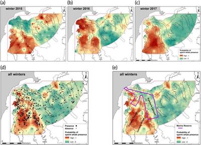
You can imagine the power that tools like this can have on marine spatial planning, fisheries management, and understanding the complex relationships between animals and their habitats. In the example above, they were able to note the foraging preferences on both the fine and coarse spatial scale. Guerra even finds that sperm whales will change their behavior, diet, and foraging locations in response to seasonal variability in prey. GAMs, in this instance, were able to produce relatively accurate predictions even in the highly complex ecological relationships existing in these marine systems.
I have created a table describing the aims and the results in a few other recent marine mammal papers that utilize GAMs:
| Paper | Purpose | Results |
|---|---|---|
| Thorne, et al. (2019) | Use mixed effects GAMs to predict pilot whale distribution and using these predictions to determine when and where long-line fisheries by-catch is a risk to this species | The models performed relatively well and were strongly correlated to the independent pilot whale bycatch observations used to ultimately validate the models generalizability. |
| Guazzo, et al. (2019) | Characterize the acoustic and visual records of gray whale migration & evaluate signals influencing migration | The GAMs revealed that migration in gray whales may be attributed more to intrinsic factors (age, pregnancy, etc.) rather than extrinsic factors (ocean temperature, sea ice, etc.) |
| Currie, et al. (2021) | Quantify a suite of humpback behavioral responses to vessel disturbance characteristics | Energetically demanding avoidance strategies are used in response to vessel disturbance. Vessel proximity and approach method were both major contributors to changes in behavior, but determining exact responses from a single event is often very complex. |
| Fraiser, et al. (2021) | Incorporate visual and acoustic data together with GAMs and Neural Networks to try and leverage the spatial and temporal benefits of each dataset without compromising predictability | Of the species distribution models, the joint acoustic and visual survey models performed best for two of the three species modeled. GAMS and the Neural Networks had pros and cons relating to computation power requirements, data structure limitations, and interpretability. |
| Warlick, et al. (2020) | Coupled with a Bayesian stable isotope mixing model, GAMs were used to determine seasonal variations in stable isotope values across age, sex, and pod of orcas | GAMs show seasonal C-13 enrichment in the summer as well as interannual variability in the N-15 ratios depending on the pod. There are multiple probable causes for this that relate to prey consumption and prey isotopic composition. |
| Baines, et al. (2020) | Use GAMs and MaxEnt to predict four cetacean species distributions using remotely sensed and static geographic predictors | GAMs for some species, possibly with stronger habitat preference, performed better than MaxEnt models and GAMs for other species. Overall, this paper outlines the strengths and limitations associated with different modeling structures with different species that may be behaviorally distinct. |
| Guerra, et al. (2021) | Investigate the foraging distribution of sperm whales, the characteristics of favorable foraging habitat, and how these factors change seasonally | Seafloor depth, thermal stratification in the water-column, and slope gradient and orientation all predict foraging sperm whale habitat use. Differences in seasonal habitat follow known changes in prey fluctuations in distribution and abundance. |
GAM Application in R
This section is coming soon, stay tuned!
Conclusion
If you have any questions, comments, or if you’ve found any errors, please contact me! I’ve added a technical resources section to explore more uses of GAMs in R.
Resources
- Frasier, et al. (2021) Cetacean distribution models based on visual and passive acoustic data. https://www.nature.com/articles/s41598-021-87577-1.
- Plourde, et al. (2016) Canadian Science Advisory Secretariat (CSAS Research Document).
- Becker, et al. (2020) Performance evaluation of cetacean species distribution models developed using generalized additive models and boosted regression trees. https://doi.org/10.1002/ece3.6316.
- Jacobson, et al. (2022) Quantifying the response of Blainville’s beaked whales to U.S. naval sonar exervises in Hawaii. https://doi.org/10.1111/mms.12944
- Currie, et al. (2021) The impact of vessels on humpback whale behavior: the benefit of added whale watching guidelines. https://doi.org/10.3389/fmars.2021.601433
- Thorne, et al. (2019) Predicting fisheries bycatch: a case study and field test for pilot whales in a pelagic longline fisheries. https://doi.org/10.1111/ddi.12912
- Lammers, et al. (2023) The occurrence of humpback whales across the Hawaiian archipelago revealed by fixed and mobile acoustic monitoring. https://doi.org/10.3389/fmars.2023.1083583
- Pedersen, et al. (2019) Hierarchical generalized additive models in ecology: an introduction with mgcv. https://doi.org/10.7717/peerj.6876
- Clark, et al. (2022) Dynamic generalized additive models (DGAMs) for forecasting discrete ecological time series. https://doi.org/10.1111/2041-210X.13974
R/Technical Resources
- Spatial Data Science - GAM Chapter
- Dr. Noam Ross Open Source Course - Generalized Additive Models in R
- Centre De La Science De La Biodiversité Du Québec- GAM Chapter in R Workshop
- R Bloggers - Solving Problems with GAMs
- Michael Clark Blog - GAM Online Workshop